Topics in Astrodynamics

Topics in Astrodynamics builds a mathematical foundation for understanding and analyzing artificial Earth satellite orbits, to include Earth escape and flyby trajectories. Its chapters first deal with the classical orbital elements, and then address the fundamental problem of satellite tracking: how to calculate ground traces and look angles, given the orbital elements of an artificial Earth satellite. Element set transformations and Gaussian orbit determination are then treated.

Orbital perturbations are dealt with via the topics of Cowell (numerical) orbit propagation, variation of parameters, and general perturbation theory. The final chapter addresses the fundamental problem of space surveillance: how to calculate an accurate state vector for the orbit of an artificial Earth satellite, given radar or optical observations (or some mix of both), and an initial estimate of the state vector at some epoch.

The book complements currently available works on celestial mechanics ("orbital mechanics applied to celestial bodies") by applying orbital mechanics to the approximately 10,000 artificial Earth satellites whose orbital elements are to be found in the satellite catalog of North American Aerospace Defense Command (NORAD) in Colorado Springs, Colorado U.S.A.

The book's author states, "Topics in Astrodynamics captures that which is worth passing along from what I myself have learned, worked out, and taught, both as an author and as a user of computer software for orbital analysts, over a space career that has spanned more than three decades."

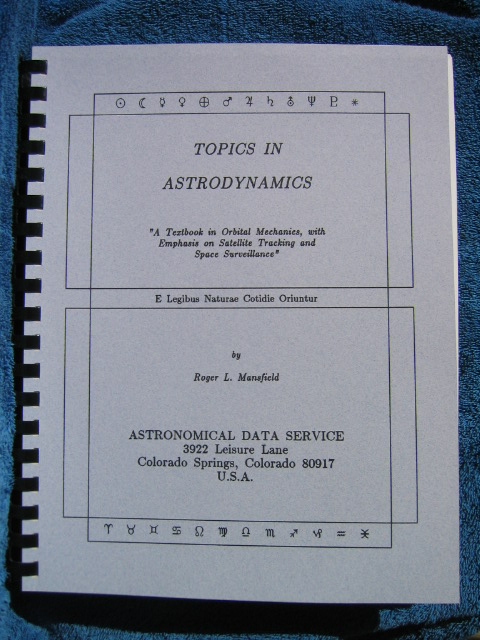
Topics in Astrodynamics was typeset as a "standard LaTeX book" using MacKichan Software's Scientific Word; see http://www.mackichan.com. Its 378 pages are sized at 8.5" by 11" and are bound between soft covers by means of a 1-1/8" diameter, 19-ring GBC plastic comb binding. See below for an actual photo of the book and a complete summary of the book's contents.

TOPICS IN ASTRODYNAMICS

Title Page i
Copyright Page ii
Dedication iii
Note on Typeset Manuscript iv
Preface v
Table of Contents ix
List of Figures xvii

Chapter 1. Introduction and Review 1
1.1 Scope 1
1.2 Review of Elementary Mechanics 2
1.2.1 Basic Definitions 2
1.2.2 Newton's Laws of Gravitation 3
1.2.3 Kepler's Laws 5
1.2.4 Work, Energy, and Conservative Forces 5
1.3 Review of the Conic Sections 8
1.3.1 Polar Transformations and Standard Form 8
1.3.2 Conic Sections and Conic Paths 9
1.4 Suggested Reading 12

Chapter 2. The Two-Body Problem 15
2.1 Equations of Relative Motion 15
2.2 Conservation Theorems 17
2.2.1 Conservation of Energy 17
2.2.2 Conservation of Angular Momentum 18
2.3 Solution of the Relative Equations 19
2.3.1 Proof of Kepler's First Law 21
2.3.2 Proof of Kepler's Second Law 25
2.3.3 Proof of Kepler's Third Law 26
2.4 The Flight Path Angle 28
2.5 Position in the Orbit Plane 29
2.5.1 Perifocal Coordinates and the Eccentric Anomaly 29
2.5.2 Kepler's Equation and the Mean Anomaly 32
2.5.3 Newton-Raphson Solution of Kepler's Equation 34
2.5.4 Orbital Position as a Function of Time 35
2.6 Useful Formulas for an Elliptical Orbit 35
2.7 Suggested Reading 37

Chapter 3. Celestial Sphere and ECI Coordinates 39
3.1 Need for an Inertial Reference Frame 39
3.2 The Celestial Sphere 4
3.3 The ECI Reference Frame 42
3.4 Celestial Coordinates and Transformations 43
3.5 Suggested Reading 44

Chapter 4. Rotation Matrices and Applications 45
4.1 Orthogonal Rotation 45
4.2 The EFG-to-ECI Transformation 48
4.3 The Euler Angle Transformation 51
4.4 Suggested Reading 53

Chapter 5. Orbital Elements & Orbit Propagation 55
5.1 Orbital Elements 55
5.2 Velocity in the Orbit Plane 58
5.3 Orbit Propagation 60
5.4 Summary Algorithm for Elliptical Orbit 61
5.5 Modification for an Orbit of Low Eccentricity 63
5.6 Suggested Reading 63

Chapter 6. Dynamical Time Conversion 65
6.1 Sidereal Time 66
6.2 Solar Time 68
6.3 Atomic Time vs. Universal Time 71
6.4 Newcomb's Formula 72
6.5 Suggested Reading 73

Chapter 7. Ground Traces and Look Angles 75
7.1 The Figure of the Earth 76
7.2 Geocentric and Geodetic Latitude 78
7.3 Subpoint Latitude and Height 80
7.4 East Longitude 83
7.5 Look Angles and Slant Range 85
7.6 Suggested Reading 87

Chapter 8. Element Set Transformations 89
8.1 Cartesian-to-Classical Transformation 90
8.1.1 Calculation of a, e, and M 90
8.1.2 Calculation of i, Omega, and omega 92
8.2 Nodal Orbital Elements 94
8.2.1 Transformations Involving Nodal Elements 94
8.2.2 Orbit Propagation Using Nodal Elements 95
8.2.3 Summary Algorithm 100
8.3 Equinoctial Orbital Elements 101
8.3.1 Transformations Involving Equinoctial Elements 102
8.3.2 Orbit Propagation Using Equinoctial Elements 103
8.3.3 Summary Algorithm 109
8.4 Summary 110
8.5 Suggested Reading 112

Chapter 9. Gaussian Orbit Determination 113
9.1 Closed-Form f and g Series 115
9.2 Derivation of Gauss's Method 116
9.2.1 Area Ratio of Sector to Triangle 118
9.2.2 The First Equation of Gauss 119
9.2.3 The Second Equation of Gauss 122
9.2.4 Iteration for E₂ - E₁ and Solution for a 124
9.3 Summary Algorithm for Gauss's Method 126
9.4 Applications of Gauss's Method 127
9.4.1 Artificial Earth Satellite Orbit Determination 127
9.4.2 Interpolation on Ephemerides 128
9.4.3 Determination of an Avoidance Trajectory 128
9.5 Critique of Gauss's Method 129
9.6 Suggested Reading 130

Chapter 10. Cowell Propagation 133
10.1 Classification of Perturbative Accelerations 136
10.2 Conservative Accelerations 137
10.2.1 Earth's Gravity 137
10.2.2 Sun, Moon, and Major Planet Gravity 140
10.3 Non-Conservative Accelerations 141
10.3.1 Solar Radiation Pressure 141
10.3.2 Atmospheric Drag 144
10.4 Numerical Propagation 145
10.4.1 Reduction of Order 146
10.4.2 Runge-Kutta Numerical Integration 147
10.4.3 Application to the Cowell Problem 148
10.5 Summary 150
10.6 Suggested Reading 150

Chapter 11. Variation of Parameters 153
11.1 Lagrange's Planetary Equations 155
11.1.1 Lagrange's Brackets 157
11.1.2 Lagrange's Brackets for the Classical Elements 158
11.1.3 Substitution of M for M₀ 164
11.2 Transformation to Other Variables 165
11.3 Gauss's Form of Lagrange's Equations 167
11.4 VOP for Earth's Equatorial Bulge 170
11.5 VOP for Atmospheric Drag 172
11.6 Numerical Integration 175
11.7 Concluding Remarks 176
11.8 Suggested Reading 177

Chapter 12. General Perturbation Theory 179
12.1 Kozai's Method 181
12.2 First-Order, Secular Perturbation Theory 185
12.3 Chebotarev's Method for Small e 187
12.4 Modeling the Drag Acceleration 188
12.4.1 Secular Changes in a and e 188
12.4.2 Two Key Assumptions 191
12.5 Orbit Propagation with Mean Elements 192
12.6 Calculation of Time Elapsed Since Epoch 196
12.7 Concluding Remarks 198
12.8 Suggested Reading 199

Chapter 13. Launch Profiles and Nominals 201
13.1 Calculating Launch Nominal Elements 202
13.1.1 Computation of Omega and M at Injection 203
13.1.2 Computation of a-bar, Given r_p or H_p 208
13.1.3 Computation of i and D_I from Az_I and Converse 209
13.1.4 The Case Where omega is not Specified 210
13.2 Moving Epoch to Revolution Zero 210
13.2.1 Purpose of Moving Epoch 210
13.2.2 Propagation of Mean Elements 211
13.2.3 Computation of n-bar and Delta-t_I 212
13.3 The January 1.0 UTC Liftoff Convention 214
13.3.1 When a Cooperative Launch is Delayed 214
13.3.2 Non-Cooperative Launch Assessment 216
13.4 Polar Orbiter Launch Practice 217
13.5 Hypothetical NPOESS Launch Example 219
13.6 Orbital Maneuvers 224
13.6.1 One-Impulse Maneuvers 224
13.6.2 Multiple-Impulse Maneuvers 225
13.6.3 Application of the Hohmann Transfer 228
13.7 Geostationary Launch Practice 228
13.8 Hypothetical GOES Launch Example 231
13.9 Suggested Reading 235

Chapter 14. Escape and Flyby Trajectories 237
14.1 Uniform Path Mechanics 238
14.1.1 Stumpff's c-Functions 239
14.1.2 Conic Elements 249
14.1.3 Uniform Propagation of Conic Elements 250
14.1.4 Kepler's Equation Revisited 260
14.1.5 Propagation of Position and Velocity 263
14.2 Gaussian Orbit Determination 268
14.3 Goodyear's State Transition Matrix 272
14.4 Suggested Reading 275

Chapter 15. Differential Correction 277
15.1 Batch Least Squares 277
15.1.1 Optical Residuals and Partials 282
15.1.2 Radar Residuals and Partials 285
15.1.3 The H Matrix 290
15.1.4 Summary Algorithm 294
15.1.5 H^TWH Matrix Accumulation 296
15.2 Variant Orbit Partials 297
15.3 Escape Trajectory Example 299
15.4 State Space Analysis 306
15.4.1 Batch Filter for Two-Body Trajectory 306
15.4.2 Batch Filter for Perturbed Trajectory 308
15.4.3 Batch DC vs. Batch Filter 310
15.4.4 Statistical Orbit Determination 311
15.5 Suggested Reading 312

Appendix A. Astrodynamic Notation 313
A.1 Chapter 1 - Introduction and Review 314
A.2 Chapter 2 - The Two-Body Problem 315
A.3 Chapter 3 - Celestial Sphere and ECI Coordinates 316
A.4 Chapter 4 - Rotation Matrices and Applications 316
A.5 Chapter 5 - Orbital Elements and Orbit Propagation 316
A.6 Chapter 6 - Dynamical Time Conversion 317
A.7 Chapter 7 - Ground Traces and Look Angles 318
A.8 Chapter 8 - Element Set Transformations 319
A.9 Chapter 9 - Gaussian Orbit Determination 319
A.10 Chapter 10 - Cowell Propagation 320
A.11 Chapter 11 - Variation of Parameters 321
A.12 Chapter 12 - General Perturbation Theory 321
A.13 Chapter 13 - Launch Profiles 322
A.14 Chapter 14 - Escape and Flyby 322
A.15 Chapter 15 - Differential Correction 323
A.16 References 323

Appendix B. Astrodynamic Constants 325
B.1 Canonical Units 327
B.2 Precession and Nutation 328
B.3 References 329

Appendix C. Spherical Trigonometry 331
C.1 Spherical Law of Sines 333
C.2 Spherical Law of Cosines for Sides 333
C.3 Spherical Law of Cosines for Angles 334
C.4 Napier's Rules 334
C.5 Earth Satellite Injection 335
C.6 Azimuth Direction from a Point 336
C.7 Radio Wave Propagation 339
C.8 Suggested Reading 339

Appendix D. Chebotarev's Method 341
D.1 Lagrange's Equations for Small e 341
D.2 The Disturbing Potential for Small e 342
D.3 First-Order Perturbations 344
D.3.1 Mean Argument of Latitude 346
D.3.2 Secular and Periodic Updating 348
D.4 Orbit Propagation Procedure 348
D.4.1 Preliminary Calculations 348
D.4.2 Convert to Nodal Elements 349
D.4.3 Update for Secular Perturbations 350
D.4.4 Update for Periodic Perturbations 351
D.4.5 Transform to Position and Velocity 352
D.5 Suggested Reading 352

Index 353

Back to Top

Roger L. Mansfield is a space professional with more than 30 years of military, industrial, and academic experience. He began his space career as an orbital analyst for the Defense Meteorological Satellite Program (DMSP) in August 1967, when he was assigned to the 4000th Support Group at Offutt Air Force Base, Nebraska. (Offutt AFB is now the home of Headquarters U.S. Strategic Command.)

As principal engineer for space surveillance applications at Ford Aerospace and at Loral Command & Control Systems, Mr. Mansfield led efforts to develop algorithms and software for the 427M Space Surveillance Center (1976-1981) and for the Space Defense Operations Center (1982-1996) in Air Force Space Command's Cheyenne Mountain Air Force Station. As assistant professor at CU-Colorado Springs, he taught astrodynamics and numerical methods to graduate space engineers working for Lockheed Martin Astronautics at the Waterton Canyon facility near Denver, Colorado.

Mr. Mansfield's personal webpage at http://mathcadwork.astroger.com/ describes just a few of the Mathcad worksheets he has constructed since 1997 to solve problems in the mechanics of Earth orbital, escape, flyby, and interplanetary trajectories. His freely downloadable Mathcad worksheets provide live, graphical examples of many of the algorithms and procedures in his book. And the worksheets employ familiar mathematical notation, not ASCII program code.

With "Nicolaus Copernicus" at AGI's 15th Annual Monte Carlo Night, April 2015

Back to Top

The book's intended audience has been: military and civilian members of the U.S. Air Force; other U.S. governmental departments and agencies dealing with space; the U.S. space industry; professors and students of space engineering.

Back to Top

Mathsoft used to publish a monthly online newsletter, the Mathcad Advisor, for Mathcad users. In the issue dated 08/12/2005 there was an article, "Tracking the International Space Station (ISS)," that showed how to use the Mathcad Animation quicksheet, "Rotating Earth," to display a ground trace for the ISS over any orbital revolution of interest.

The article explained how to generate a ground trace of a satellite’s orbit around the Earth using Two-Line Elements (TLE) from NORAD’s Space Track website. It then showed how to superimpose the ground trace onto both 2D and 3D renderings of Earth's surface.

The article also provided links to the downloadable Mathcad 11 worksheets and data file that generate the ground trace and its associated 2D and 3D plots. They are GroundTrace.mcd, WorldPlot.mcd, and the data file trace.prn. Visit* http://www.mathcad.com and click on "Resources", then on "Tech Advisor Newsletter", and finally on "Mathcad Advisor - 8/12/2005". Or, just click on: http://www.mathcad.com/resources/newsletter/default.asp?cID=108.

*Sadly, when PTC took Mathcad over from Mathsoft (this is discussed in Mathcad Worksheets by Astroger) the Mathcad Advisor archive seems to have been lost. So I cannot link you to the "Tracking the International Space Station (ISS)" article, but I'd probably respond favorably to a polite e-mail request for the worksheets. Both .mcd and .pdf formats are available.

Back to Top

Mathsoft used to publish a monthly online newsletter, the Mathcad Advisor, for Mathcad users. In the issue dated 11/05/2003 there was an article, "Topics in Astrodynamics and Kepler's Laws," that provided some further information about the book and its treatment of astrodynamics, satellite tracking, and space surveillance.

The article also linked to a worksheet on Kepler's laws of planetary motion that you could download and animate using Mathcad 11. The worksheet tells step-by-step how to do the animation. Go to* http://www.mathcad.com and click on the Mathcad Advisor link, then click on the 11/05/2003 issue. Look for the "Featured User" sidebar. Or, try clicking on this direct link: http://www.mathcad.com/resources/newsletter/default.asp?cID=87.

*Sadly, when PTC took Mathcad over from Mathsoft (this is discussed in Mathcad Worksheets by Astroger) the Mathcad Advisor archive seems to have been lost. So I cannot link you to the "Topics in Astrodynamics and Kepler's Laws" article. But all is not lost -- read on.

To request the "Kepler's Laws of Planetary Motion" worksheet, send an e-mail to the address at the end of this webpage and state what version of Mathcad you have. My reply will include, as an attachment, a copy of the Kepler's laws worksheet, saved for the version of Mathcad that you have (must be Mathcad PLUS 6 or later).

Don't have Mathcad at all? A PDF version of the Kepler's laws worksheet is available, and is readable with Adobe's Acrobat Reader. You won't be able to animate the worksheet without Mathcad, but you will be able to see the math equations and the graphical plot. And you will see firsthand that a Mathcad worksheet is readable and useful even to a non-user of Mathcad. E-mail your request to the address at the end of this webpage.

Back to Top

Here is a listing of the author's supplemental Mathcad worksheets, as further described at http://mathcadwork.astroger.com/. These worksheets integrate major segments of the book's math into working algorithms. They conform closely to the notation of the book and take full advantage of Mathcad Professional's programming capabilities.

But please note: the original purpose of writing these worksheets was not to illustrate the material in the book, but rather, to communicate results on contemporary astrodynamic problems. Many of the algorithms in the book are not covered in these worksheets. Moreover, some of the worksheets address topics not discussed in the book

1. Ephemeris of a Comet Via Uniform Path Mechanics (UPM). This worksheet applies the UPM theory as derived in Chapter 14 of the book. It ties together material from the first seven chapters of the book. And it showcases many of the programming features of Mathcad that were new when the worksheet was constructed (1997).

2. Herget's Method for an Asteroid. Herget's method of orbit determination has Gauss's "two position vector and time of flight" method built in. Thus this worksheet applies material from Chapter 9 of the book as well as building upon ideas in Chapters 3 and 6.

3. Orbit Propagation via State Space Analysis. This worksheet applies material discussed in Chapters 10 and 15 of the book.

4. Effect of a Radial Impulse on a Circular Orbit. This worksheet illustrates a special kind of orbital maneuver, the purely radial impulse. Orbital maneuvers are discussed further in Chapter 13 of the book.

5. Herget's Method with Cassini's Earth Flyby. Worksheet #2 applies Herget's method to determination of the orbit of an asteroid moving in the gravitational field of the sun. This worksheet applies Herget's method to determination of the orbit of the space probe Cassini, assumed to be "in orbit" around Earth. This worksheet uses observations taken when Cassini was actually just flying by planet Earth, and thereby receiving a gravity assist from Earth, on its journey to the planet Saturn and its moon Titan.

6. Sun Altitudes for Sextant Practice. This worksheet develops a quantitative model of Earth's orbit around the sun (and thus of the sun's "orbit" around Earth), and shows how to calculate sextant measurements using this model. It has value for predicting the sun's altitude and azimuth at any time on any date, and applies many of the ideas treated in the book (note that the "elevation" of an artificial Earth satellite, as described in Chapter 7 of the book, is the same as the "altitude" of a celestial body such as the sun).

7. Sun-Sight Solutions Without Tables. This worksheet shows how to calculate one's Earth-fixed position using sextant measurements and an accurate watch, without having to use sight reduction tables. Like Worksheet #6, it applies many of the ideas treated in the book, most notably ideas developed in Chapters 3, 6, and 7.

8. Rectilinear Two-Body Motion ("Earth Falls Into the Sun"). An application of two-body mechanics for which Chapters 2 and 14 of the book provide good background reading.

9. Gauss's Angles-Only Method with "Killer Asteroid". Chapter 9 of the book treats Gauss's "two position vector and time of flight" orbit determination method. This worksheet extends that method to work for three angles-only observations of an asteroid.

10. Tracking Data Reduction for Galileo's Earth 1 Flyby. This worksheet illustrates the material in Chapter 15 of the book, and can be modified easily to reproduce the test case for the NEAR spacecraft's Earth escape of 1996 February 17, as provided in Chapter 15 of the book.

11. Calculating the Photoperiod in Plant Physiology. The photoperiod is the duration of daylight at a given location on Earth's surface, as a function of latitude and season. This new (as of April 14, 2004) pair of worksheets is not about astrodynamics per se, but rather, is about the connection between dynamical astronomy (i.e., Earth's rotational and orbital motions) and plant physiology.

The worksheets show how to calculate the photoperiod and its diurnal rate, both numerically and analytically. (The photoperiod is calculated numerically by subtracting the time of sunrise from the time of sunset each day. The photoperiod diurnal rate is calculated numerically by subtracting the photoperiod for one day from the photoperiod for the next. By implementing rigorous numerical calculations in Mathcad, I was able to deduce simple analytical formulas for the photoperiod and its diurnal rate; these formulas are derived in the worksheets.)

12. Modeling Blackbody Radiation. 2005 was the "World Year of Physics" and it marked the 100th anniversary of Albert Einstein's publication of papers on the photoelectric effect, Brownian motion, and the special theory of relativity. All four papers on these three topics appeared in the year 1905.

But modern physics, i.e., modern quantum physics really began in 1901, when Max Planck propounded the notion that material bodies, but especially blackbodies*, emit and absorb thermal radiation in discrete quanta of energy, rather than continuously. (*A blackbody is an ideal body in thermal equilibrium that absorbs all incident radiation and re-emits it as light energy distributed over the entire electromagnetic spectrum.)

Planck's hypothesis of quantized absorption and emission of radiation made it possible for him to derive a radiation law that applies to blackbody emission at all wavelengths and all frequencies, a universal law that succeeds in spectral regions where the prior radiation laws of Rayleigh, Jeans and Wien had failed. Planck received the Nobel Prize in physics in 1918 for his quantum theory of radiation.

The Mathcad 12 worksheet, "Modeling Blackbody Radiation," revisits how Max Planck integrated the blackbody radiation curve for an arbitrary Kelvin temperature, T, over all possible wavelengths of thermal emission, to arrive at the Stefan-Boltzmann law. The Maple symbolic processing capability of Mathcad is invoked at key points of the derivation and Bernoulli numbers are used to evaluate the infinite series that is crucial to the derivation. Finally, Mathcad's X-Y Plot capability is used to plot the blackbody radiation curve for 2.725 degrees Kelvin.

Planck's radiation law is not just of historical interest. In 1964 Arno Penzias and Robert Wilson discovered radio noise emanating from all directions of the sky that is consistent with thermal emission from a blackbody at an equilibrium temperature of just a few degrees Kelvin. They deduced in 1965 that this radio noise is the cosmic microwave background (CMB). For this they were awarded a Nobel Prize in 1978 [1].

By the 1960s there were two competing theories of the origin of the cosmos, the "steady state" theory and the "Big Bang" theory. Existence of the CMB was predicted by the Big Bang theory, but not by the steady state theory. So when the CMB was found by Penzias and Wilson, most physicists and astronomers came to accept the Big Bang theory and to reject the steady state theory.

More recently, the Cosmic Background Explorer (COBE) spacecraft measured the CMB in all directions of space, from space (i.e., from Earth orbit). Its measurements of energy density vs. frequency fit almost perfectly on Planck's radiation curve for a blackbody at 2.725 degrees Kelvin. But small "ripples" in energy density were in fact found; these are believed to be evidence of variations in the early universe's energy density. Since these variations are thought to have seeded star and galaxy formation, it would have been a setback for the Big Bang theory had they not been found.

REFERENCE

[1] Mather, John C. and Boslough, John, The Very First Light, Basic Books, New York, 1996; pp. 49-50 and 64. John Cromwell Mather was the original proposer and project scientist for the COBE mission. The COBE satellite was launched on November 18, 1989.

Back to Top

It is believed that there is sufficient material in Topics in Astrodynamics for a two-semester course sequence, especially if some of the problems and computer projects are worked out in class. It is assumed that each of the two semesters includes fifteen weeks of instruction, with three contact hours per week (45 lecture hours per semester). Here is what is recommended.

Astrodynamics I. Fundamentals of Orbital Mechanics. This course will include astronomical timekeeping and reference frames; two-body motion in the orbit inertial and Earth-centered inertial (ECI) reference frames; ground traces and look angles; orbital elements and element set transformations; Gaussian preliminary orbit determination; Cowell (numerical) orbit propagation with perturbations.

Teach Chapters 1-10 during the first semester. Spend the first six contact hours teaching "Mathcad as an Electronic Scratchpad" and "Mathcad as a Programming Language". (This might seem like a lot to cover in a single semester, but I have taught Chapters 1-12 in a one-semester course without Mathcad.)

Astrodynamics II. Analytical Methods and Orbit Determination. This course will include derivations of Lagrange's Planetary equations and Gauss's form of Lagrange's equations, with applications that include variation of parameters (VOP) for J₂ and the drag acceleration; general perturbation theory; launch profiles and launch nominal elements; escape and flyby trajectories; batch least squares differential correction using radar and optical observations; batch least squares filter for a perturbed trajectory.

Teach Chapters 11-15 during the second semester.

Problem sets and computer projects that support such a two-semester course sequence are included on the same CD-ROM that contains the electronic edition of the book. They are included on a supplemental CD-ROM that accompanies the print edition of the book.

See Space Ornithology for related information about Earth satellite tracking as a hobby.

Back to Top

As noted above, my course design calls for the first ten chapters of Topics in Astrodynamics to be taught in Astrodynamics I, and for the remaining five chapters to be taught in Astrodynamics II. The first eight of twelve problem sets and the first two of eight computer projects go with Astrodynamics I. The remaining four problem sets and six computer projects go with Astrodynamics II. Thus, each of the two courses has ten homework assignments.

The computer projects were conceived as Mathcad worksheet-writing assignments. Top-level descriptions are as follows, with relevant book chapters given in parentheses.

Project 1. Given a set of heliocentric ecliptic orbital elements for the planet Jupiter, generate a two-body ephemeris good for the year 2004. Use the orbital elements with the Mathcad worksheet winupm.mcd to generate geocentric equatorial sky coordinates (right ascension and declination), so that you can locate Jupiter among the stars in the night sky. This project applies material from Chapters 1-5. It also uses the worksheet winupm.mcd, which is now bundled with the book. The full title of the winupm.mcd worksheet is "Geocentric Equatorial Ephemeris of a Comet via UPM".

Project 2. Given a tracking radar's geodetic coordinates, transform two topocentric (Rho, Az, El) observations of a satellite to ECI coordinates (Ch. 7). Use Gauss's method to calculate the satellite's ECI velocity at the time of the first observation (Ch. 9). Transform position and velocity to classical orbital elements (Ch. 8). The "Gauss's Angles-Only Method with Killer Asteroid" worksheet is a good reference here. The file name is 1997 XF11.mcd. It is now bundled with the book.

Project 3. Generate a two-body ephemeris for an artificial Earth satellite via the orbital elements specified for the project. This part is very similar to Project #1, but (a) the Gaussian gravity constant is for Earth rather than for the Sun, and (b) while Jupiter's mass relative to that of the Sun must be considered in Project #1, the artificial Earth satellite's mass relative to that of Earth can be ignored for this project. Output an ephemeris matrix whose rows consist of time, position, and velocity, and a second ephemeris matrix whose rows consist of time and the classical orbital elements. Your work on Project #2 will help you here (reuse your implementation of the cartesian-to-classical elements transformation).

Now use Cowell propagation (Ch. 10) with Mathcad's built-in Rkadapt integrator to generate the same two sets of ephemeris matrices by adaptive Runge-Kutta integration. When the two-body ephemerides obtained via orbital elements agree with the two-body ephemerides obtained via numerical integration, add in the perturbative accelerations due to the J₂ term in the geopotential. Your two-body ephemeris matrix of orbital elements will, of course, contain classical orbital elements for which only the mean anomaly changes with time. But your perturbed ephemeris matrix of orbital elements will show you how the orbital elements change with time as the result of the J₂ perturbations.

Project 4. Implement Variation of Parameters (VOP) for the classical elements (Ch. 11), for the same test case as for Project #3, and account for the perturbative accelerations due to J₂. Output an ephemeris matrix that consists of time, position, and velocity. Output an ephemeris matrix that consists of time and the classical orbital elements as well. Your results with VOP for classical elements should agree with your results from Project #3 to within about a tenth of a kilometer, in magnitude of position vector difference at the last time point of the integration span.

Project 5. Propagate a set of NORAD Two-Line mean elements (TLE)* using the GP1 model from Chapter 12. Output a ground trace matrix of times, latitudes, east longitudes, and heights above Earth's reference spheroid (Ch. 7). Given the geodetic latitude, east longitude, and height above the reference spheroid of a ground station, generate a look angles matrix (Ch. 7) that includes times, azimuths, elevations, and slant ranges. When you get the worksheet working correctly, put a filter in your look angles generator function so that only look angles matrix rows with a positive elevation angle are displayed.

*Back in the mid-1980s, Dr. T.S. Kelso started a Bulletin Board Service (BBS) to make unclassified NORAD TLE available to members of the international space community via telephone line and modem. His service continues on today in the form of the CelesTrak WWW website, accessed via http://celestrak.com.

The CelesTrak WWW website is valuable not only as a source for up-to-date NORAD TLE, but also as a source for code and documentation relating to NORAD's SGP and SGP4 orbit propagation models. Two more items of interest about the website: (a) Dr. Kelso wrote a series of columns on satellite tracking and space surveillance for the now-defunct Satellite Times. His articles have been archived at the CelesTrak WWW website. They are essential reading for satellite orbital analysts. (b) The CelesTrak WWW website describes commercial satellite tracking software packages and provides links to their websites.

Project 6. Given an actual "Element Set 1" for a Molniya communications satellite, and historical information about Molniya launches from Plesetsk, work out the launch azimuth, time of flight from parking orbit injection to final orbit injection, the parking orbit's classical orbital elements, and the scalar delta-V, in km/sec, for injection into the final orbit (Ch. 13).

Project 7. Modify Project #2 so that Gauss's method works for parabolic and hyperbolic paths (Ch. 14). The worksheets and data files associated with "Tracking Data Reduction for Galileo'sEarth 1 Flyby" provide test data for this project. They are now bundled with the book.

Project 8. Given observations from optical and radar trackers, differentially correct the nominal state vector for the NEAR spacecraft's Earth escape trajectory (Ch. 15). You should obtain results that match exactly the test case data given on p. 300 of Topics in Astrodynamics. The worksheets and data files associated with "Tracking Data Reduction for Galileo's Earth 1 Flyby" are key resources for this project. They are now bundled with the booki.

The specifications for these computer projects are included on the same CD-ROM that contains the electronic edition of the book. They are included on a supplemental CD-ROM that accompanies the print edition of the book. And note that all twelve of the Mathcad Worksheets by Astroger are now bundled with the book.

See Space Ornithology for related information about Earth satellite tracking as a hobby.

Back to Top

Topics in Astrodynamics commenced publication on October 6, 2003, by Astronomical Data Service, with postal mailing address as follows.

Astronomical Data Service is a member of the American Astronomical Society (AAS), the American Astronautical Society (AAS), the Mathematical Association of America (MAA, the Air Force Association (AFA), the Air Force Historical Foundation, and the Denver Astronomical Society.

Astronomical Data Service conducts research in orbital mechanics, with particular emphasis on dynamical astronomy and astrodynamics. For further information, see The Astroger* Webpages.

(c) 2004-2018 by Astronomical Data Service. Last updated 2018 October 17.

Accesses: